Written by Warren Alphonso, advised by Ntwali Bashige.
Once realized, quantum computers would be an intellectual and engineering triumph, success in turning Nature’s powerful and mysterious laws into computational power. If our current understanding of quantum mechanics holds up, it would mean the ability to efficiently simulate any physical process.
But it might take decades to build a quantum computer powerful enough to catch up with classical computers after their 50-year headstart.
A question I’ve been trying to answer since I started studying quantum computing concerns its near-term usefulness: what exactly can near-term quantum computers tell us about the world that our classical physical heuristics can’t? I don’t have a great answer yet, but this question is the guiding principle for the following post.
Most near-term useful work will probably use variational algorithms. This project explores the most well-known of the variational algorithms: the Variational Quantum Eigensolver (VQE). We’ll use the VQE to analyze a fundamental model in condensed matter physics, the Hubbard model.
You’ve noticed the length of this post by now. It is intentional; I’ve favored a long, winding, wandering, uncertain path as the search for uses of a quantum computer. Let’s get started! [1] Note to the prospective reader: I’ve done my best to only assume you’ve read the four essays at QuantumCountry. Another thing: I don’t know much quantum mechanics, so instead of pretending like things make sense when I don’t understand them, I’ll explicitly say “This is true by magic” as a reminder that we’re assuming something without understanding it.
Table of Contents
- A quantum mechanical solid!
- Generalizing to the Hubbard model
- The Hubbard Hamiltonian
- The Jordan-Wigner transformation
- Mott gap
The Hubbard model
It is almost like Nature knows you are blatantly cheating, but she gives you a passing grade anyway.
— Ntwali Bashige
A quantum mechanical solid!
When do we need to use quantum computers to analyze solids? Quantum computers are based on quantum mechanics, so we can intuit that materials whose properties and behavior are so quantum mechanical that we can’t hope to approximate them with classical methods will be good candidates for demonstrating the usefulness of quantum computers.
But what solids fit this description? From Griffiths’ Introduction to Quantum Mechanics,
Problem 1.21: In general, quantum mechanics is relevant when the de Broglie wavelength of the particle in question is greater than the characteristic size of the system (\(d\)). In thermal equilibrium at (Kelvin) temperature \(T\), the average kinetic energy of a particle is \[\frac{p^2}{2m} = \frac{3}{2} k_B T\] (where \(k_B\) is Boltzmann’s constant \(1.380 \times 10^{-23} \mathrm{J \cdot K^{-1}}\)), so the typical de Broglie wavelength (\(\lambda = h / p\)) is \[\lambda = \frac{h}{\sqrt{3m k_B T}}\] where \(h\) is Planck’s constant \(6.626 \times 10^{-34} \mathrm{J \cdot s}\).
The purpose of this problem is to anticipate which systems will have to be treated quantum mechanically, and which can be safely described classically.
The lattice spacing in a typical solid is around \(d=0.3 \mathrm{nm}\). Find the temperature below which the free1 electrons in a solid are quantum mechanical. Below what temperature are the nuclei in a solid quantum mechanical? Use sodium as a typical case. Moral: The free electrons in a solid are always quantum mechanical; the nuclei are almost never quantum mechanical.
1In a solid the inner electrons are attached to a particular nucleus, and for them the relevant distance would be the radius of the atom. But the outermost electrons are not attached, and for them the relevant distance is the lattice spacing. This problem pertains to outer electrons.
[2] We don’t know what or why the de Broglie wavelength is useful. We just assume that’s correct. Treat it like magic.
We want to solve \(\lambda > 3 \times 10^{-10} \mathrm{m}\). To do that, we need to choose some value for mass \(m\) to plug in, so that the inequality is only a function of temperature \(T\). The problem recommends using sodium:
Solving \(\lambda > d\): \[ \frac{h}{\sqrt{3m k_B T}} > 3 \times 10^{-10} \qquad \rightarrow \qquad \frac{h}{3 \times 10^{-10} \sqrt{3m k_B}} > \sqrt{T} \qquad \rightarrow \qquad \frac{h^2 \cdot 10^{20}}{9 \cdot 3 m k_B} > T \]
Solving for electrons:
The mass of an electron is \(m = 9.109 \times 10^{-31} \mathrm{kg}\). Plugging in \(h\), \(m\), and \(k_B\), we get \[T < 1.2935 \times 10^{5} = 129350 \mathrm{K}\]
For some perspective on this result, the surface of the sun is about \(6000 \mathrm{K}\). Almost everywhere on Earth satisfies the above temperature inequality; the electrons in sodium always require quantum mechanical treatment.
Solving for the nucleus:
Sodium has atomic number 11, which means it has 11 protons. The most common isotope of Sodium is 23Na, which has 12 neutrons. Because the mass of an electron is about a thousand times smaller than the mass of a proton or a neutron, we’ll ignore them when calculating mass. With only protons and neutrons, our total mass is \[11 \cdot 1.672 \times 10^{-27} + 12 \cdot 1.674 \times 10^{-27} \mathrm{kg} = 3.848 \times 10^{-26} \mathrm{kg}\]
Plugging in \(h\), \(m\), and \(k_B\), we get \[T < 3.062 \mathrm{K}\]
This temperature is near-zero. The lowest natural temperature recorded on Earth is \(184 \mathrm{K}\), so the above inequality is almost never met. The nucleus can usually be treated with classical methods.
Our takeaway is that outer electrons must be analyzed quantum mechanically while nuceli can be well approximated classically. We’ll focus on solids whose outer electrons majorly determine their properties.
Why are electrons important?
It’s not clear why we should care about the outer electrons of atoms in a solid.
But since we want to do something useful with quantum computers that can’t be done with classical computers, this seems like a good thread to follow!
Generalizing to the Hubbard model
The problem we’re attacking is: how do the outer electrons in a solid affect the properties of the entire solid?
We’ll need some way to model this problem before we can start making progress. Let’s make some simplifying assumptions:
- Assume the atoms (nuclei) aren’t moving. We can model this as a
lattice of fixed sites.
- The mass of an electron is more than a thousand times smaller than the mass of a proton. Since the nucleus is made up of protons and neutrons, we’re justified in thinking only of movement relative to the nucleus, i.e. we assume the nucleus is stationary.
- Assume the atoms only have one electron orbital. The Pauli
exclusion principle states that each orbital can have a maximum of 2
electrons: a spin-up electron and a spin-down electron.
- This might seem like leap at first, because atoms can have many electron orbitals. But because we know that the outer electrons must be treated quantum mechanically, we may ignore any inner orbitals. While there can be multiple outer electron orbitals, we choose to only consider one outer orbital. I don’t have a great justification for this; it’ll just make calculations easier if we focus on the simplest case.
- Assume 2 electrons interact with each other only if they’re
in the same orbital.
- Interaction strength is determined by proximity: two electrons interact very strongly if they’re very close. We’ve decided to only consider the strongest interactions.
- Assume electrons can only hop to another atom if that atom is
directly adjacent to their current atom.
- It’s easiest and most common for electrons to hop to the nearest orbital, so we’re only considering these hopping terms.
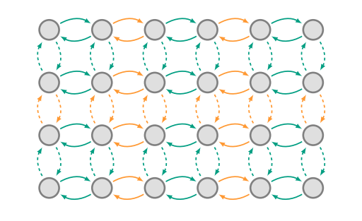
These 4 assumptions define the Hubbard model of solids. Pictorially, we can represent the Hubbard model on a 2-dimensional lattice as:
We’re making good progress, but we’ll need more than a purely visual understanding of our model.
Defining creation and annihilation operators
From our 4 assumptions above, there seem to be 2 main ideas we need to express about the behavior of free electrons: the kinetic energy of an electron moving from site to site, and the potential energy of 2 electrons interacting with each other if on the same site.
Here, I introduce a concept that isn’t motivated but extremely useful: the creation and annihilation operators. These arise from studying the quantum harmonic oscillator. [3] I recommend Lecture 8 and Lecture 9 of MIT OCW 8.04 Spring 2013.
Since we’re describing electrons, the creation and annihilation operators have fermionic anticommutation relations. In other words, for two fermions on sites \(j\) and \(k\), with spins \(\sigma\) and \(\pi\), we have:
\[ \Large \begin{split} & \{ a_{j \sigma}, a^\dagger_{k \pi} \} = \delta_{jk} \delta_{\sigma \pi} \\ & \{ a_{j \sigma}^\dagger, a_{k \pi}^\dagger \} = 0 \\ & \{ a_{j \sigma}, a_{k \pi} \} = 0 \end{split} \]
[4] By the way, these curly braces are called the anticommutator operator. It’s just a shorthand for the sum of products of two operators: \(\{ A, B \} = AB + BA\). }
We can derive some interesting properties of operators that obey the above relations, namely the Pauli exclusion principle.
For now, I’ll quickly summarize what you need to know about these operators.
We call \(a^\dagger\) the creation operator and \(a\) the annihilation operator. Their names reflect that \(a^\dagger_{j \sigma}\) creates a fermion on site \(j\) with spin \(\sigma\) while \(a_{j \sigma}\) destroys a fermion on site \(j\) with spin \(\sigma\).
I said I don’t know why these relations hold, but we can try to think about how we might have derived them by ourselves. We want some relation that makes it clear that \(a^2\) and \(a^{\dagger^{2}}\) are both nonsense, since we can’t have two fermions of the same spin in the same place. Since we’re working in a vector space, we can set these both equal to \(0\), which means that applying either of these operations destroys our whole vector space. Notice another way of writing \(a^2 = 0\) is \(2a^2 = \{ a, a \} = 0\) which is the exact anticommutation relation we have. The same logic works for \(a^\dagger\). This explain two of the three relations above.
How could we have come up with the first relation?
Recall from the quantum harmonic oscillator that \(a \ket{n} = \sqrt{n} \ket{n-1}\) and \(a^\dagger \ket{n} = \sqrt{n+1} \ket{n+1}\). Let’s enforce the rule that \(n\) can only be \(0\) or \(1\). Notice that if \(n\) is constrained to those values, then \(\sqrt{n} = n\) and \(\ket{n-1} = \ket{1-n}\). With this we can write \[ a \ket{n} = n \ket{1-n} \qquad a^\dagger \ket{n} = (1 -n) \ket{1-n}\]
Now what is \((aa^\dagger + a^\dagger a) \ket{n}\)? It simplifies to \((2n^2 -2n + 1)\ket{n}\). Plugging in \(n=0\) and \(n=1\) results in the same thing: \(2n^2 -2n+1 = 1\), which means we can write that \(\{ a, a^\dagger \}\) is always equal to 1, and we get our first commutation relation!
One last useful operator: the number operator \(\hat{n} = a^\dagger a\): \[\hat{n} \ket{n} = a^\dagger a \ket{n} = a^\dagger (n \ket{1 - n}) = n^2 \ket{n} = n \ket{n}\] As you can see, it’s behavior is to multiply a state by the number of fermions that occupy it. When it’s clear, I’ll use \(n\) instead of \(\hat{n}\) to denote the number operator.
The Hubbard Hamiltonian
The Hamiltonian of a system is the operator that represents its energy, \(H = KE + PE\), where \(KE\) is kinetic energy and \(PE\) is potential energy. {% annotate The Hamiltonian’s eigenstates are the possible resulting states when we measure a system, each eigenstate’s corresponding eigenvalue is that state’s energy, and the Hamiltonian tells us exactly how a system evolves with time according to the Schrödinger equation. Why this operator turns out to be so important is a much harder question. For now, it’s magic. Using the language of creation and annihilation operators, we can write the Hamiltonian as \[ H = -t \sum_{ \braket{j, k} \sigma} ( a^\dagger_{j \sigma} a_{k \sigma} + a^\dagger_{k \sigma} a_{j \sigma} ) + U \sum_j n_{j \uparrow} n_{j \downarrow} \]
The first term represents the kinetic energy. It’s also called the tunneling term. Notice the notation \(\braket{j, k}\). I use this to denote we’re summing over adjacent sites \(j\) and \(k\). The second term represents the potential energy. It’s also called the interaction term. Notice it’s nonlinear - we only add \(U\) if there are 2 electrons on a site.
This notation should seem weird. We almost never add unitary matrices in quantum computing, because the resulting sum isn’t generally unitary. But Hamiltonians must be Hermitian, and it’s easy to see that the sum of Hermitian matrices is also Hermitian. Still, what does a sum of matrices physically mean? If we multiply some vector by this matrix, we’re acting on it with the kinetic and potential energy matrices and our result is a sum of the results. So maybe we can intuitively think of a sum of Hermitian matrices as two processes happening simultaneously to our state. [5] This explanation is in Scott Aaronson’s recenly-published lecture notes on Quantum Information Science.
Notice our interaction term is only relevant if there are 2 electrons on some sites. If have \(n\) total sites, then we can have a maximum of \(2n\) electrons, 1 spin-up and 1 spin-down on each site according to the Pauli exclusion principle. If we have less than or equal to \(n\) electrons, we can order them so that we never have any interaction energy \(U\) by placing at most one electron on each site. This isn’t exactly a physical behavior because it means all those configurations have the same energy. To fix this, we’ll add a chemical potential energy \(\mu\) which scales with the total number of electrons: [6] I don’t have a good explanation of why the chemical potential is important. It seems to be how “accepting” the system is of additional particles. It adds a linear potential term, so that we don’t have a potential only if we have 2 electrons.
\[ H = -t \sum_{ \braket{j, k} \sigma} ( a^\dagger_{j \sigma} a_{k \sigma} + a^\dagger_{k \sigma} a_{j \sigma} ) + U \sum_j n_{j \uparrow} n_{j \downarrow} - \mu \sum_j (n_{j \uparrow} + n_{j \downarrow}) \]
The Jordan-Wigner transformation
We’ve got analytic and visual ways to think of our model now, but how can we represent it on a quantum computer? Notice that our Hamiltonian calculates energy based on where electrons are, so it’s keeping track of the location of electrons. If there are \(n\) possible sites in our lattice, then we have \(2n\) possible locations an electron could be: each site can have an up electron and a down electron. We call each of the \(2n\) locations a spin-orbital. Now that we’ve simplified our model to deciding whether or not an electron is in a spin-orbital, we can represent it with \(2n\) qubits, one for each spin-orbital. If we order our \(2n\) qubits by having the \(n\) up spin-orbitals be represented in the first \(n\) qubits, and then the \(n\) down spin-orbitals be represented in the last \(n\) qubits, if the \(j_\uparrow\)-th spin-orbital has an electron, then the \(j\)-th qubit is \(\ket{1}\), and if the \(j_\downarrow\)-th spin-orbital doesn’t have an electron, then the \(n + j\)-th qubit is \(\ket{0}\).
Now that we have this figured out, we need some way to encode our creation and annihilation operators into qubit operators. There are 3 main ways of doing this, but we’ll focus on the Jordan-Wigner transformation. [7] The 2 other popular ways to encode are the Bravyi-Kitaev and parity encodings. These are more complex than the Jordan-Wigner encoding but more useful in some situations.
The Jordan-Wigner transformation is very intuitive, and we can stumble across it ourselves. We need \(a^\dagger\) to convert \(\ket{0} \rightarrow \ket{1}\) and \(\ket{1} \rightarrow 0\), while \(a\) must convert \(\ket{1} \rightarrow \ket{0}\) and \(\ket{0} \rightarrow 0\). Since qubits are 2-dimensional and we’ve specified the transforms of 2 basis vectors, we’ve completely defined the operators. Specifically, \[ a^\dagger = \begin{bmatrix} 0 & 0 \\ 1 & 0 \end{bmatrix} = \frac{X - iY}{2} \qquad a = \begin{bmatrix} 0 & 1 \\ 0 & 0 \end{bmatrix} = \frac{X + iY}{2} \]
I’ve left out the subscripts, but remember that these operators are defined on the space of \(2n\) qubits. So in reality, \(a^\dagger_j = I \otimes ... \otimes \frac{X - iY}{2} \otimes ... \otimes I\) and similarly for \(a_j\), which just means that we apply the identity to all other qubits and leave them alone.
But these don’t satisfy the anticommutation relations above! We require that \(a^\dagger_j a^\dagger_k = - a^\dagger_k a^\dagger_j\) for any \(k\) and \(j\). However, with our current encoding, we instead have \(a^\dagger_j a^\dagger_k = a^\dagger_k a^\dagger_j\). (Try some examples to understand why this is the case.)
We need some way to to apply a \(-1\) factor whenever we switch the order of the operators. Recall that the Pauli matrices satisfy \(AB = -BA\). If we prepend our operator with tensor products of the remaining unused Pauli matrix \(Z\), then we can use this property to get the desired behavior. [8] This article by Microsoft is a great resource.
This is the Jordan-Wigner transform. We use the above formulation for \(a^\dagger\) and \(a\), then prepend the operator with Pauli \(Z\)s and append a sequence of identity operators \(I\). In other words, \[ \begin{align} a^\dagger_1 &= \frac{X - iY}{2} \otimes I \otimes I \otimes ... \otimes I \\ a^\dagger_2 &= Z \otimes \frac{X - iY}{2} \otimes I \otimes ... \otimes I \\ &\vdots \\ a^\dagger_{2n} &= Z \otimes Z \otimes Z \otimes ... \otimes \frac{X -iY}{2} \end{align} \]
We can guess that these matrices become huge by looking at the chains of tensor products. For example, if we have a 4 site Hubbard model, we’d need 8 qubits for the JW transformation which means our Hilbert space has dimension \(2^8 = 256\). For a 10 site model our vectors have dimension \(2^{20} = 1048576\). This gets out of hand quickly!
Mott gap
Most chemistry problems are concerned with finding the eigenstates and eigenvalues of the Hamiltonian. The most important eigenstate is the state corresponding to the lowest eigenvalue. We call this eigenstate the ground state and its corresponding eigenvalue the ground state energy. The name indicates that the eigenstates are configurations of the system that have a particular energy, specifically their corresponding eigenvalues. Why is the ground state so important? Because the system will tend toward its lowest energy state over time. Most systems spend the vast majority of their time in their ground state, so if we can understand its properties well, we can understand most of the behavior of the system.
Before we decide to use a quantum computer to figure out some properties of the Hubbard model, let’s try to make some progress with paper-and-pencil.
Some materials that were predicted to conduct electricity turned out to be insulators, especially at low temperatures. These are called Mott insulators, and their behavior is due to electron-electron interactions (like \(U\) in the Hubbard model) that classical theories don’t account for. We’ll use the Hubbard model to understand this!
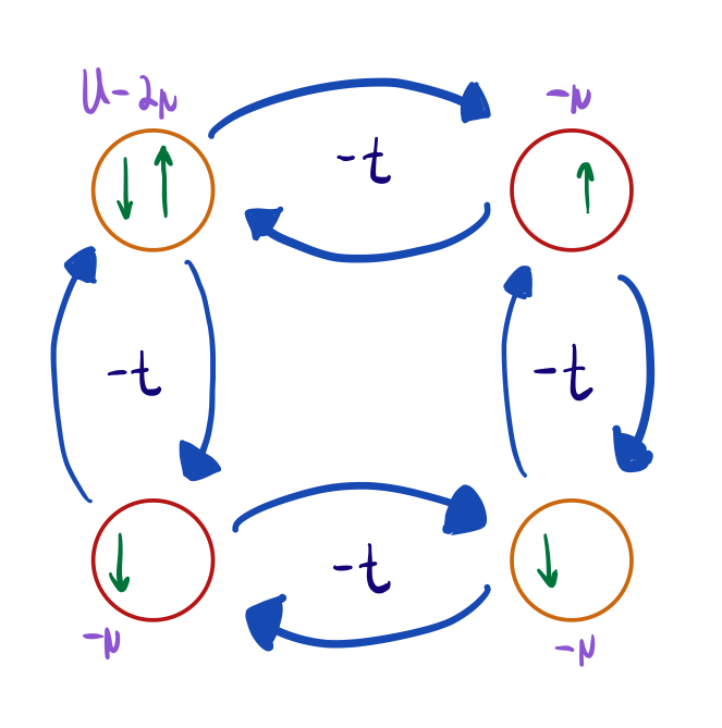
Let’s do a simple version: the one-site case. Since there’s only one site, we have no hopping terms. Since electrons aren’t moving, it’s easy to see that we have 4 eigenstates: \(\ket{0}, \ket{\uparrow}, \ket{\downarrow}, \ket{\uparrow \downarrow}\), where \(\ket{0}\) indicates we have no electrons, and the arrows indicate the existence of an electron with that particular spin. By plugging in these eigenstates into the Hamiltonian, we can see that their eigenvalues are \(0, -\mu, -\mu, U - 2\mu\), respectively.
With this, we can calculate the partition function of the system. [9] I don’t yet understand how the partition function is so powerful, but we’ll see below that it allows us to calculate some important quantities. It’s true by magic.
It’s defined as \[Z = \mathrm{Tr } (e^{-\beta H}) = \sum_i \bra{i} e^{-\beta H} \ket{i} = \sum_{i= 0, \uparrow, \downarrow, \uparrow \downarrow} e^{-\beta E_i} \braket{i \vert i} = 1 + 2e^{\beta \mu} + e^{-\beta U + 2 \beta \mu} \] where \(\beta = \frac{1}{k_B T}\).
The partition function lets us calculate expectations easily. For any observable \(m\), \(\braket{m} = Z^{-1} \mathrm{Tr } (m e^{-\beta H})\). We will find the density \(\rho = \braket{n}\) for number operator \(n\). Using the previous formula, we have \[ \begin{align} \rho &= \braket{n} = Z^{-1} \mathrm{Tr } (ne^{-\beta E_i}) = Z^{-1} \sum_i e^{-\beta E_i} \braket{i \vert n \vert i} = Z^{-1} (0 + e^{\beta \mu} + e^{\beta \mu} + 2 e^{-\beta (U - 2 \mu)} ) \\ &= 2 \cdot Z^{-1} ( e^{\beta \mu} + e^{2 \beta \mu - \beta U}) \end{align} \]
I graphed the density \(\rho\) for temperatures \(T = 0.5\) and \(T = 2\) K. Try changing the potential energy \(U\). Can you explain the result based on the Hubbard Hamiltonian?
Clearly there is some plateau where \(\rho\) becomes 1 at low temperatures when \(U\) becomes large. Upon reflection, this isn’t all that mysterious. Up until we have half-filling (1 electron on every site), \(U\) doesn’t affect the energy calculation at all because it’s only relevant if there are 2 electrons on a site. But once we hit this limit, the cost to add an additional electron is exactly \(U - \mu\). Unless \(\mu\) is about equal to \(U\), we’re stuck at half-filling. This is the exact behavior we see in the graph.
What’s harder to explain is why this doesn’t occur at high temperatures. Indeed, the effect is almost completely gone when the temperature increases by 1.5 Kelvin! I don’t have an answer to this yet.
Earlier, I motivated this by telling you about the Mott insulator. Let’s see if our graph gets us closer to a solution. We can think of a solid that conducts electricity as one in which electrons are able to move freely. Mott insulators, then, are materials in which electrons stop moving freely at low temperatures.
Our graph tells us that at low temperatures the Hubbard model is stuck at half-filling. Does this mean electrons can’t move? Yes, if every site has one electron then an electron hopping to a nearby site would incur a penalty of \(U\). Electrons don’t move around, and the material stops conducting electricity.
But wait, this is just a guess! Our graph is only for a single site Hubbard model. Having to account for tunneling terms and more sites would make finding the eigenvalues/vectors (and thus calculating \(\rho\)) much harder.
This is the first problem we’ll try solving with a quantum computer. All we need to do is calculate \(\rho = \braket{n}\). In the Jordan-Wigner transformation, we encode each spin-orbital in a qubit, so all we have to do to find \(\rho\) is measure each qubit.
Exploring the Variational Quantum Eigensolver (VQE)
In this section, we’ll learn how to use VQE to learn properties of the \(2 \times 2\) Hubbard model. People tend to focus on finding the ground state energy to high accuracy with VQE, but I honestly still don’t know why this is such an important quantity and why we need such high accuracy. We’ll find the ground state energy anyway because we get it for free when we do VQE, but I’m more interested in the ground state itself. Once we finish running VQE and find the ground state, we can analyze its properties.
In this section, we will discuss the measurement of interesting physical observables. The total energy… is the least interesting quantity. We will instead focus on densities and density correlations, kinetic energies, Green’s functions and pair correlation functions.
— Wecker et. al., Section 6 of 1506.05135
Representing the \(2 \times 2\) Hubbard model
I’ll be using the OpenFermion
software package for most of this post. OpenFermion is an open-source
project that makes working with quantum chemistry much easier. [10] I originally planned to write my own
code for representing and simulating the Hamiltonian for the Hubbard
model, but it was wildly inefficient. My computer couldn’t handle
anything more than a \(2 \times 2\)
Hubbard Hamiltonian, probably because I was storing the entire matrix.
For the \(2 \times 2\) case this
translates to a \(256 \times 256\)
matrix. OpenFermion doesn’t use this approach, opting to store strings
of creation and annihilation operators or scipy.sparse
matrices. OpenFermion is built by Google, so they’ve made it
easy to integrate with their own quantum computing library Cirq. We’ll be using Cirq
as well later on.
FermiHubbardModel instance
from our lattice. The format for the tunneling and interaction
coefficients is a little weird — check out the documentation
for an explanation.
And that’s it. We can access the actual Hamiltonian with
hubbard.hamiltonian().
VQE Primer
I’ll give only a short hand-wavy explanation of the VQE algorithms; for a more in-depth understanding I recommend Michał Stęchły’s article.
The VQE algorithm uses a principle in quantum mechanics called the variational principle, which states that \[ \bra{\psi} H \ket{\psi} \geq E_0\] where \(E_0\) is the ground state energy and \(\ket{\psi}\) is any state vector. A simple way to see that this inequality holds: we can write any state vector \(\ket{\psi}\) as a linear combination of eigenvectors \(\ket{\psi} = \sum_i a_i \ket{E_i}\), so \(H\) acting on this linear combination multiplies each eigenvector by its eigenvalue \(E_i\) and then we take the inner product with the initial state \(\ket{\psi}\) which had norm 1 so we’re left with $_i a_i E_i $ of each eigenvector, which is clearly minimized if \(\ket{\psi} = \ket{E_0}\), the ground state.
The variational principle tells us that if we minimize \(\bra{\psi} H \ket{\psi}\) we’ll find the ground state. Machine learning and optimization techniques have been getting pretty good in the past few years; the insight of VQE is that we should use classical optimization techniques with a quantum computer. How? We create a parameterized circuit, which changes its gates based on a few parameters that a classical optimizer chooses.
The number of parameters increases very quickly. This paper found an ansatz that can reach every single state in the 2-qubit state space; the ansatz has 24 parameters. Our Hubbard model is represented on an 8-qubit state space. The strategy of an ansatz that can reach every single state would probably require thousands of parameters and be incredibly hard to optimize. That’s why choosing a good ansatz is very important.
Once we have a state, how do we find \(\bra{\psi} H \ket{\psi}\)? The only way we can extract information from a quantum circuit is through measurement so we have to rephrase this quantity as a measurement somehow.
Lemma 0: The Pauli tensors form a basis for all Hamiltonians.
Proof: The Pauli matrices are: \[ I = \begin{bmatrix} 1 & 0 \\ 0 & 1 \end{bmatrix} \quad X = \begin{bmatrix} 0 & 1 \\ 1 & 0 \end{bmatrix} \quad Y = \begin{bmatrix} 0 & -i \\ i & 0 \end{bmatrix} \quad Z = \begin{bmatrix} 1 & 0 \\ 0 & -1 \end{bmatrix} \]
Any 2-dimensional Hermitian operator can be written as: \[H = \begin{bmatrix} a & b \\ b^* & c \end{bmatrix}\] where \(a, c\) are real. We can define a linear combination of the Pauli matrices as: \[ a_0 I + a_1 X + a_2 Y + a_3 Z = \begin{bmatrix} a_0 + a_3 & a_1 - i a_2 \\ a_1 + i a_2 & a_0 - a_3 \end{bmatrix} \] for real \(a_i\). Notice the upper-right and lower-left elements are complex conjugates of each other which is what a Hermitian matrix requires. The upper-left and lower-right values can be any real number, we just choose \(a_0\) to be the midpoint between the desired two real numbers and then \(a_3\) the distance from the midpoint to the desired number.
This means the Pauli matrices form a basis for 2-dimensional Hermitian matrices. Then we simply use the definition of the tensor product, which states that for any two vector spaces \(V_1\) and \(V_2\) with basis \(\{ e_i \}\) and \(\{ f_j \}\), the tensor product \(V_1 \otimes V_2\) is a vector space with basis \(\{ e_i \otimes f_j \}\).
All Hamiltonians are Hermitian and have dimension \(2^n\) where \(n\) is the number of qubits they act on, so all Hamiltonians can be written as a linear combination of Pauli tensors.
\(\blacksquare\)
Thus, we can write \(\bra{\psi} H \ket{\psi}\) as a linear combination of Pauli tensors, like \(\bra{\psi} \frac{1}{2} X \otimes Y \otimes \cdots \otimes Z + \frac{1}{2} ... \ket{\psi}\).
This is useful because we can compute these with measurements. I’ll do a 1-qubit example: suppose we wanted to get \(\bra{\psi} Z \ket{\psi}\). We can write \(\ket{\psi}\) as a linear combinations of \(Z\)’s eigenvectors: \(\ket{\psi} = c_0 \ket{0} + c_1 \ket{1}\). Now, \[\bra{\psi} Z \ket{\psi} = \Big( c_0^* \bra{0} + c_1^* \bra{1} \Big) \Big( c_0 \ket{0} - c_1 \ket{1} \Big) = \lvert c_0 \rvert^2 - \lvert c_1 \rvert^2 \] Hey, \(\lvert c_0 \rvert^2\) is the probability we measure \(\ket{0}\) and \(\lvert c_1 \rvert^2\) is the probability we measure \(\ket{1}\), so we can find these values by doing a bunch of measurements and averaging our results. This can be extended to multiple-qubit states by measuring \(\ket{00}\), etc., and can be extended to other Pauli operators by changing basis so any Pauli operator’s eigenvectors are \(\ket{0}\) and \(\ket{1}\).
As a reminder, the VQE algorithm requires us to specify 3 things: an ansatz, an initial state, and some initial parameters. We’ll choose them in the next few sections.
The Variational Hamiltonian Ansatz
Adiabatic evolution
A mysterious result in quantum mechanics is the adiabatic theorem. To quote Wikipedia: “A physical system remains in its instantaneous eigenstate if a given pertubation is acted on it slowly enough and if there is a gap between the eigenvalue and the rest of the Hamiltonian’s spectrum.”
Suppose we have two Hamiltonians \(H_A\) and \(H_B\), and we know an eigenstate of \(H_A\) to be \(\ket{\psi_A}\). Then we can define a new Hamiltonian \(H(s) = (1 - s) H_A + s H_B\). Notice that as \(s\) goes from \(0\) to \(1\) our time-dependent Hamiltonian goes from \(H_A\) to \(H_B\).
The adiabatic theorem tell us that if we evolve \(\ket{\psi_A}\) by \(e^{-itH(s)}\) while slowly changing \(s\), the final resulting state will be the corresponding eigenvector of \(H_B\). (It will be clearer later what I mean by “corresponding eigenvector.”) This is useful if one Hamiltonian is diagonal, or at least easy to diagonalize, because then we can easily find its ground state. Then we adiabatically evolve this ground state to get the ground state of another Hamiltonian that is perhaps harder to diagonalize.
I haven’t proven the adiabatic theorem because I don’t know how to yet. We’re just assuming it’s true for now. Regardless, let me try to make things more concrete with an example.
The Schrödinger equation is \[ i \frac{d \ket{\psi}}{dt} = H \ket{\psi} \] which means, for time-independent \(H\), the solution is \[ \ket{\psi(t)} = e^{-i H t} \ket{\psi(0)} \] where we evolve for time \(t\).
Suppose we choose \(5\) discrete times: \(H(0), H(.25), H(.50), H(.75), H(1)\). At each time step, we’ll simulate for \(t=1\). Then, if an eigenvector of \(H_A\) is \(\ket{\psi_A}\), an eigenvector of \(H_B\) is: \[\ket{\psi_B} = e^{-i H(1)} e^{-i H(0.75)} e^{-i H(0.50)} e^{-i H(0.25)} e^{-i H(0)} \ket{\psi_A}\]
Of course, this only works if we choose sufficiently many discrete values for \(s\) and a short enough time \(t\).
The adiabatic theorem tells us this will work only if we choose sufficiently many values of \(s\) and a short enough time \(t\). I wish I could prove some bounds for these, but I can’t yet. 😞
Here’s an example with \(2 \times 2\) Hamiltonians. We’ll choose \(H_A = Z\) and \(H_B = X\).With n = 5, we get res = [0.299+0.668j,
-0.137-0.668j] and np.dot(H_B, res) gives us
res = [-0.137-0.668j, 0.299+0.668j], which isn’t quite an
eigenvector.
However, if we set n = 50, we get res = [
0.713-0.043j, -0.698+0.043j], which is very close to the
eigenvector of the Pauli \(X\) matrix
with eigenvalue \(-1\). We started with
the ground state of \(H_A\) and ended
in the ground state of \(H_B\), just
like the adiabatic theorem predicts!
Let’s try one last example. Instead of \(H_B = X\), this time we’ll use \(H_B = \begin{bmatrix} -5 & 0 \\ 0 & 4
\end{bmatrix}\). When we use the same parameters as before
(n = 50, t = 1), we get res = [0,
0.92175127+0.38778164j]. This is very close to [0,
1] which is the eigenvector with eigenvalue \(4\). We didn’t get the ground
state! What went wrong?
We can get some intuition by plotting the eigenvalues of \(H(s)\) as we increase \(s\):
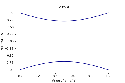
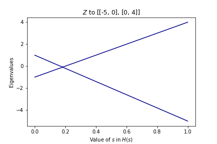
In the first graph, there is no crossing of the eigenvalues. We started with the lowest eigenstate of \(Z\) and ended in the lowest eigenstate of \(X\). In the second graph, however, there is a crossing! Though we started in the lowest eigenstate of \(Z\), we didn’t end up in the lowest eigenstate of the final matrix. Instead, it’s almost like we “followed the line” that shows up in the graph. If we wanted to get the ground state of the final matrix, we would have had to start in the \(+1\) eigenstate of \(Z\).
Keep this in mind! It means we have to choose which state we start in carefully. We cannot simply start in the ground state everytime.
An ansatz based on adiabatic evolution
Adiabatic evolution is an interesting concept and seems very powerful — it allows us to find ground states of arbitrary Hamiltonians by starting with an easy Hamiltonian. The catch is that the change in \(s\) might have to be exponentially small.
Instead of calculating this ourselves, we can just turn it into an ansatz and let an optimizer choose the best values!
I’m going to rewrite the adiabatic evolution equation: \[ \ket{\psi_B} = \prod_s e^{-i t H(s)} \ket{\psi_A} = \prod_s e^{-i t (1-s) H_A - itsH_B} \ket{\psi_A} = \prod_k e^{\theta_{kA} H_A + \theta_{kB} H_B} \ket{\psi_A}\] where the final equality just means I’m making \(\theta_k\) a parameter that I want the optimizer to choose. If \(H_A\) and \(H_B\) commute, then we also have [11] For matrices \(A\) and \(B\), it is not generally true that \(e^{A + B} = e^A e^B\). \[\ket{\psi_B} = \prod_k e^{\theta_{kA} H_A} e^{\theta_{kB} H_B} \ket{\psi_A}\]
Here’s our strategy for the Hubbard model: we’ll set \(H_A\) to be the tunneling term and \(H_B\) to be the full Hamiltonian. This is because the tunneling term is quadratic which means that it’s a linear combination of operators that are products of at most 2 creation and annihilation operators. We have efficient algorithms to diagonalize these and easily find the eigenvalues and eigenvectors. But the interaction term (and therefore the entire Hubbard Hamiltonian) is quartic. There’s no efficient way to find its eigenspectrum.
OpenFermion has a lot of good ansatze already defined that we can
use. The two most relevant ones for the Hubbard model are
SwapNetworkTrotterAnsatz and
SwapNetworkTrotterHubbardAnsatz. The former is a generic
adiabatic evolution ansatz which has about 20 parameters per iteration
for the \(2 \times 2\) Hubbard, while
the latter is a less accurate that has 3 parameters per iteration.
After many hours of testing different configurations, I came up with
a custom ansatz that scales as 9 parameters per iteration for the \(2 \times 2\) Hubbard and has the same
accuracy as SwapNetworkTrotterAnsatz. The code is messy
because I had to make slight modifications to some methods in the
SwapNetworkTrotterAnsatz class, but it’s available here.
We’ve got our ansatz now. But we also need to choose an initial state and specify initial parameters. We’ll go over choosing an initial state in the next section.
Turns out theSwapNetworkTrotterAnsatz class (which my
custom ansatz inherits from) has a good default strategy for initial
parameters if we don’t specify one. Here’s the docstring that explains
it:
Choosing an initial state
We’ve got an ansatz and initial parameters. The final requirement for VQE is an initial state. Since our ansatz is inspired by adiabatic evolution, our initial state needs to be the ground state of \(H_A\). Since we’ve set \(H_A\) to be the tunneling term, we’re going to find its ground state.
This section has a lot of math. While working through “Elementary Introduction to the Hubbard Model,” I found the appearance of the following ideas remarkable, so I’m including them.
I highly recommend you do the math with me, but if you find that tedious, the last subsection goes over code that can just find the ground state for us. This is cheating, but since I told you quadratic Hamiltonians ground states are efficiently solvable it’s an okay place to cheat.
Position to momentum transformation
We can apply a Fourier transform to our creation operators to change from position to momentum basis:
\[a_{k\sigma}^\dagger = \frac{1}{\sqrt{N}} \sum_l e^{i k \cdot l} a_{l \sigma}^\dagger\] where \(k\) is a discrete momentum and \(l\) is a discrete position eigenstate. In \(1\)D, \(k \cdot l = kl\).
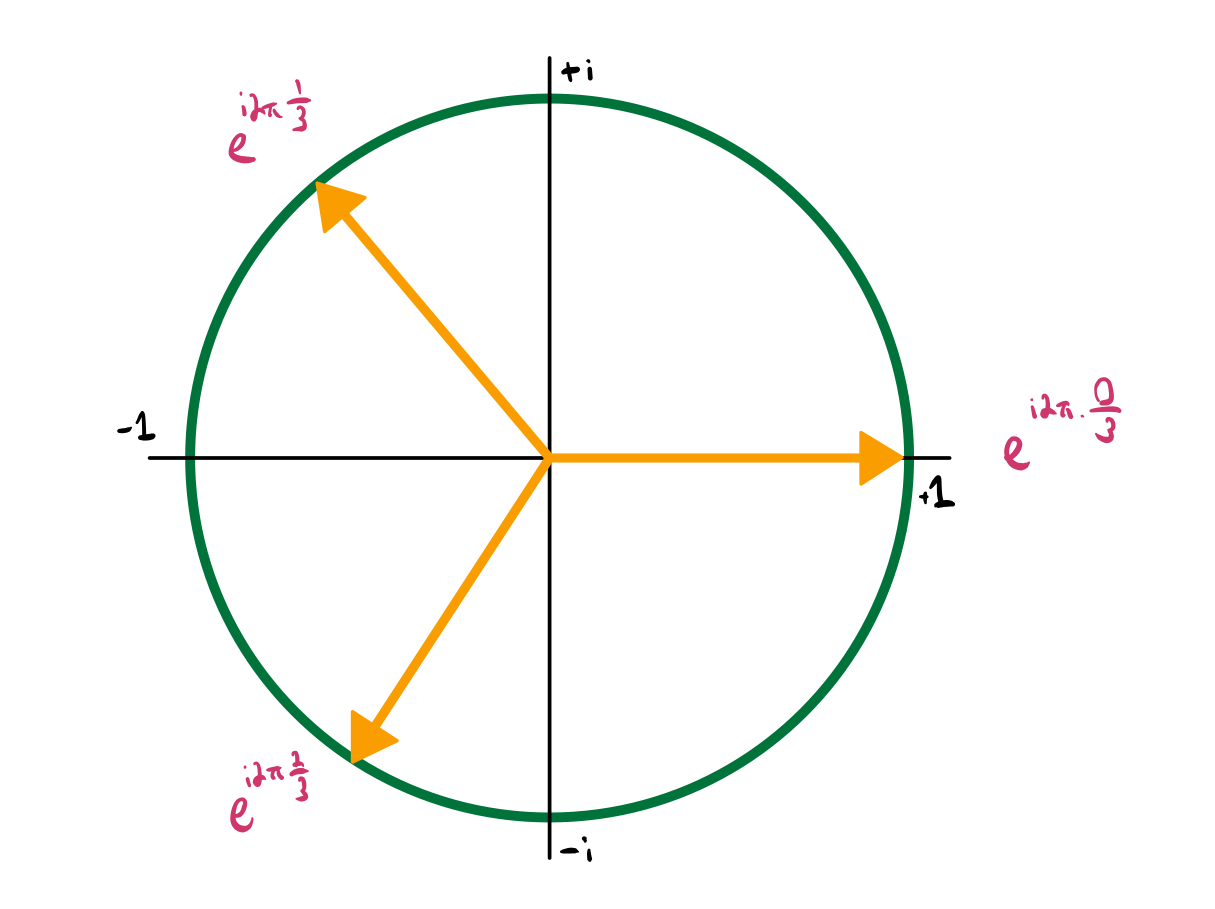
If you’re not familiar with the Fourier transorm, right now you don’t lose much by thinking of this as defining new operators as linear combinations of the old ones. Below (and in most treatments of Fourier analysis), we use the concept of \(n\)-th roots of unity, \(\omega\), which satisfy \(\omega^n = 1\).
Lemma 1: \(\frac{1}{N} \sum_l e^{i (k_n - k_m) \cdot l} = \delta_{n, m}\) where \(k_n = 2 \pi n/N\).
Proof: \[ \begin{align} \frac{1}{N} \sum_l e^{i (k_n - k_m) \cdot l} &= \frac{1}{N} \sum_l e^{i 2 \pi \frac{n-m}{N} \cdot l} \\ &= \frac{1}{N} \sum_l \omega^l \qquad \text{ which follows from setting $\omega = e^{i 2 \pi \frac{n-m}{N}}$} \\ &= \frac{1}{N} \frac{1 - \omega^N}{1 - \omega} \qquad \text{ by definition of finite geometric series} \\ &= 0 \qquad \text{ since $w^N = 1$} \end{align} \]
Of course, here we asssumed \(\omega \neq 1\), otherwise we can’t use the finite geometric series formula. In that case, \(\frac{1}{N} \sum_l 1^l = 1\). Either way, \(\frac{1}{N} \sum_l e^{i (k_n - k_m) \cdot l} = \delta_{n, m}\).
\(\blacksquare\)
Lemma 2: \(\frac{1}{N} \sum_n e^{i k_n (l - j)} = \delta_{l, j}\).
This uses the same strategy as the previous proof, so I’ll skip this proof.
These two lemmas rely on our definition of momentum as \(k_n = 2 \pi n/N\). From now on, when summing over \(k_n\) I’ll write summing over \(k\), ie \(\sum_{k_n} = \sum_k\).
\(\blacksquare\)
Lemma 3: \(a_{l \sigma}^\dagger = \frac{1}{\sqrt{N}} \sum_k e^{-i k \cdot l} a_{k \sigma}^\dagger\)
Proof: \[ \begin{align} \frac{1}{\sqrt{N}} \sum_k e^{-i k \cdot l} a_{k \sigma}^\dagger &= \frac{1}{N} \sum_{kj} e^{-i k \cdot l} e^{i k \cdot j} a_{j \sigma}^\dagger \qquad \text{ which follows by converting $a_{k \sigma}^\dagger$ to position basis} \\ &= \frac{1}{N} \sum_j a_{j \sigma}^\dagger \sum_k e^{i k \cdot (j - l)} \\ &= \sum_j a_{l \sigma}^\dagger \delta_{l, j} \qquad \text{ by Lemma 2} \\ &= a_{l \sigma}^\dagger \end{align} \]
\(\blacksquare\)
Using these relations, it’s easy to verify that the creation and annihilation operators in the momentum basis obey the fermionic anticommutation relations. I won’t do that here; most of the proof is mechanical.
Lemma 4: \(\sum_{k \sigma} a_{k \sigma}^\dagger a_{k \sigma} = \sum_{l \sigma} a_{l \sigma}^\dagger a_{l \sigma}\) for momentum \(k\) and position \(l\).
Proof:
\[ \begin{align} \sum_{k \sigma} a_{k \sigma}^\dagger a_{k \sigma} &= \frac{1}{N} \sum_{klm \sigma} e^{i k(l-m)} a_{l \sigma}^\dagger a_{m \sigma} \qquad \text{ by transforming both operators to position basis} \\ &= \frac{1}{N} \sum_{lm \sigma} a_{l \sigma}^\dagger a_{m \sigma} \sum_k e^{i k (l -m)} = \sum_{lm\sigma} a_{l \sigma}^\dagger a_{m \sigma} \delta_{l, m} \qquad \text{ by Lemma 2} \\ &= \sum_{l \sigma} a_{l \sigma}^\dagger a_{l \sigma} \end{align} \]
\(\blacksquare\)
Take a moment to make sense of this result. The sum of number operators over position is equal to the sum of number operators over momentum. Every fermion has its own position and momentum, so these are just two ways of counting up the total number of fermions. We could have predicted this property without doing the math.
The 1D tunneling term
Theorem 1: For \(U = 0\), the \(1\)D Hubbard Hamiltonian in momentum basis is \[ H = \sum_{k \sigma} (\epsilon_k - \mu) a_{k \sigma}^\dagger a_{k \sigma}\] where \(\epsilon_k = -2t \cos k\).
Proof: Our strategy will be to convert \(\sum_{k \sigma} \epsilon_k a_{k \sigma}^\dagger a_{k \sigma}\) to position basis, and then use Lemma 4 to convert \(\mu \sum_{k \sigma} a_{k \sigma}^\dagger a_{k \sigma}\) to position basis.
\[ \begin{align} \sum_{k \sigma} \epsilon_k a_{k \sigma}^\dagger a_{k \sigma} &= \frac{-2t}{N} \sum_{klm\sigma} \cos (k) e^{ik(l-m)} a_{l \sigma}^\dagger a_{m \sigma} \qquad \text{ by transfoming both operators to position basis} \\ &= \frac{-2t}{N} \sum_{lm\sigma} a_{l\sigma}^\dagger a_{m \sigma} \sum_k \cos (k) e^{ik(l-m)} \\ &= \frac{-2t}{N} \sum_{lm \sigma} a_{l \sigma}^\dagger a_{m \sigma} \sum_k \frac{1}{2} (e^{ik} + e^{-ik}) e^{ik (l-m)} \qquad \text{ by using the identity $\cos (x) = (e^{ix} + e^{-ix})/2$} \\ &= \frac{-t}{N} \sum_{lm \sigma} a_{l \sigma}^\dagger a_{m \sigma} \sum_k e^{ik(l-m+1)} + e^{ik(l-m-1)} \end{align} \]
Notice that by Lemma 2, \(\sum_k e^{ik(l-m \pm 1)} = 0\) if \(l-m \pm 1 \neq 0\), otherwise it’s \(N\). Thus, we simplify to only the adjacent terms! \[\sum_{k \sigma} \epsilon_k a_{k\sigma}^\dagger a_{k \sigma} = -t \sum_{\braket{l, m} \sigma} a_{l \sigma}^\dagger a_{m \sigma} \]
By Lemma 4, we can tack on the chemical potential term too, so we have \[H = \sum_{k \sigma} (\epsilon_k - \mu) a_{k \sigma}^\dagger a_{k \sigma}\]
\(\blacksquare\)
This took me by complete surprise. The tunneling term in the position basis looks strange because we have this awkward behavior of summing over neighbors with \(\braket{l, m}\). It’s crazy that summing over all momentum number operators and multiplying by some cosine somehow equals this awkward summation in the position basis.
This means that by switching to the momentum basis we diagonalize our tunneling term. In this basis, its eigenvectors are just \([1, 0, 0, ...], [0, 1, 0, ...]\) and its eigenvaluesu are \(\cos (k) - \mu\).
The 2D tunneling term
Extending the previous result to 2 dimensions isn’t that hard.
Theorem 2: For \(U=0\), the 2D Hubbard Hamiltonian is \[H = \sum_{k \sigma} (\epsilon_k - \mu) a_{k \sigma}^\dagger a_{k \sigma}\] where \(\epsilon_k = -2t( \cos k_k + \cos k_y)\).
Proof: The proof follows many of the same steps in the Theorem 1. Again, we’ll consider the \(\mu\) coefficient separately.
\[ \begin{align} \sum_{k \sigma} \epsilon_k a_{k \sigma}^\dagger a_{k \sigma} &= \frac{1}{N} \sum_{lm \sigma} a_{l \sigma}^\dagger a_{m \sigma} \sum_k \epsilon_k e^{i k \cdot (l-m)} \\ &= \frac{-2t}{N} \sum_{lm \sigma} a_{l \sigma}^\dagger a_{m \sigma} \sum_{k_x, k_y} e^{i k \cdot (l-m)} (\frac{1}{2}) \Big( e^{ik_x} + e^{-ik_x} + e^{ik_y} + e^{-ik_y} \Big) \\ &= \frac{-t}{N} \sum_{lm\sigma} a_{l \sigma}^\dagger a_{m \sigma} \sum_{k_x, k_y} e^{i k_x (l_x - m_x \pm 1)} e^{i k_y (l_y - m_y)} + e^{i k_x (l_x - m_x)} e^{i k_y (l_y - m_y \pm 1)} \end{align} \]
The final step follows from extending the dot product for 2 dimensions. I wrote \(\pm 1\) for the two exponentials; this means there are 4 exponentials: one with \(+1\) in the \(x\) direction, one with \(-1\) in the \(x\) direction, \(+1\) in \(y\), and \(-1\) in \(y\). Notice that these 4 terms correspond to a difference of \(1\) in a single dimension, and by Lemma 2, we get the hopping term over neighbors again.
By Lemma 4, we can attach the chemical potential term to get \[H = \sum_{k \sigma} (\epsilon_k - \mu) a_{k \sigma}^\dagger a_{k \sigma}\]
\(\blacksquare\)
Choosing the states with best overlap
We’ve shown that a change of basis exists that makes it easy to find the eigenvalues/vectors of the tunneling and chemical potential terms in the Hubbard Hamiltonian. Eearlier, we noticed that adiabatic evolution doesn’t always work if we input the ground state as our initial state. This means we’ll have to try many different eigenvectors until we find one that converges.
Here’s how we’ll approach this:
- Let \(H_A\) be the tunneling and chemical potential terms of the Hubbard Hamiltonian (the quadratic terms). Let \(H_B\) be the full Hubbard Hamiltonian.
- Create a perturbed Hamiltonian: \(H(s) = (1-s) H_A + s H_B\) for small \(s\).
- Find the ground state of \(H_B\) by brute-force. (This is cheating.)
- Find the eigenvectors of \(H(s)\) by brute-force. (This is cheating.)
- Try adiabatically evolving one of the eigenvectors of \(H(s)\) into the ground state of \(H_B\). Keep trying until we find one that works.
- This will be our starting state - if we let \(s \rightarrow 0\) we can make this arbitrarily close to a linear combination of \(H_B\)’s eigenvectors.
This seems very complicated! Why can’t be just try a bunch of \(H_A\)’s eigenvectors until we find one that works? Why do we have to introduce this perturbed Hamiltonian? The answer is that our starting state might be a linear combination of \(H_A\)’s eigenvectors. By perturbing it and then solving, we let the full Hubbard Hamiltonian influence the state we pick so we’re more likely to find the correct superposition.
Here’s code for steps 1-4:Ground state energy: -6.828
Now we’ll run adiabatic evolution on eigenvectorsv_per[:, i] until we find one that evolves to have high
overlap with gstate. Code for step 5:
Overlap with perturbed eigenvector and true ground state is: 0.942
So our starting state has 94.2% overlap with the desired ground state already. Let’s see how much better VQE can get us.
How good is this ansatz?
Now we’ve got everything we need to run VQE: an ansatz, a starting state, and some initial parameters. Before we run the algorithm, let’s step back to think about what we’re expecting to happen.
At first glance, this ansatz seems pretty terrible. A good ansatz is one that explores most of the state space fairly evenly. The VHA only has access to states which our starting state evolves into.
How can we think about this more concretely? The paper “Expressibility and entangling capability of parameterized quantum circuits for hybrid quantum-classical algorithms” goes much more in-depth into this topic, but I didn’t understand most of it. Instead, I’ll use the following:
- Define a vector \[\ket{\psi} =
\frac{1}{M} \Big( \sum_{i=1}^M R_i \ket{s} - \sum_\theta
U(\theta) \ket{s} \Big)\] where \(R_i\) are uniformly
random unitary matrices and \(U(\theta)\) is our ansatz parameterized
with \(\theta\). We’ll choose these
parameters \(\theta\) to be uniformly
distributed as well. \(\ket{s}\) is our
starting state.
- The “perfect” ansatz [12] We don’t actually use this because it would have a lot of parameters and be incredibly hard to optimize. is one that has an even chance of reaching any state vector. We can simulate this with uniformly random unitary matrices, since unitary matrices are just rotations of a vector in state space. The diagrams below offer a more intuitive understanding. Then \(\ket{\psi}\) is just the difference between our ansatz and the “perfect” ansatz.
- We’ll classify the badness of an ansatz by the norm of
\(\ket{\psi}\). The smaller the badness
value, the better our ansatz.
- Since \(\ket{\psi}\) is the difference between our ansatz and the “perfect” ansatz, the smaller the magnitude of the difference, the better the ansatz.
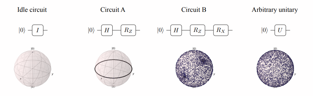
To contextualize our metric, the identity ansatz got a badness score of almost 1 while a uniformly random unitary ansatz got a badness score of about 0.06. Our ansatz got a badness score of around 0.20. This is much closer to the perfect ansatz than to the identity, which is a little surprising because our ansatz is so restricted and has very few parameters.
To be clear, this is a pretty naive metric for how good an ansatz is. Expressibility of all states isn’t nearly as important as the ansatz’ ability to reach the desired state. Regardless, it is pretty interesting that our ansatz’ badness is closer to the expressive limit than to the completely unexpressive limit.
Finding the ground state
Optimal ground state energy is -6.764
Recall the true ground state energy was
genergy = -6.828, so we were off by about 0.064.
For now, let’s see how much overlap the ground state that VHA outputted has with the true ground state.
VHA ground state and true ground state have an overlap of 0.992
99.2% overlap is great, especially since we only did 2 iterations!
Uncovering magnetism from the Hubbard model
I set out with the goal of using near-term quantum computing to actually understand something about the world that our classical heuristics couldn’t teach us, and all we’ve managed so far is a jargon-riddled journey to solving the ground state of a simple model. This section aims to cross more into the physical world. The ground state we discovered earlier is a real physical configuration of some solid; we’ll now probe the magnetic properties of that solid.
Spin and magnetism
Electron spin is deeply connected to magnetism. I don’t yet understand the physics behind this so we’ll treat it like magic.
When many electrons have the same spin, we get ferromagnetism, which means all the magnetic moments are aligned and we get a strong magnetic moment. If electron spins are balanced, they cancel each other out and we get antiferromagnetism, which means the material doesn’t have a strong magnetic moment.
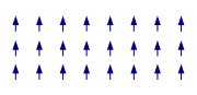

Ferromagnetic order on the left (Image source); antiferromagnetic order on the right (Image source).
So to figure out the magnetic properties of solids, we have to look at the spins of its electrons. An important quantity we’ll analyze is the local moment: \(\braket{m^2} = \braket{ (n_{\uparrow} - n_{\downarrow})^2 }\). The local moment is 0 if the site is empty or has 2 spins, and 1 otherwise. We’ll begin our analysis with the simplest case: the single site Hubbard model at half-filling.
Recall that for this case we have the partition function: \[Z = 1 + 2e^{\beta \mu} + e^{-\beta U + 2 \beta \mu} = 2 + 2e^{\beta \mu}\] where the last step follows from \(\mu = \frac{U}{2}\) as the condition for half-filling. We can write the expectation of the local moment as: \[ \begin{align} \braket{m^2} &= \braket{(n_{\uparrow} - n_{\downarrow})^2} = \braket{n_{\uparrow}} + \braket{n_{\downarrow}} - 2\braket{n_{\uparrow} n_{\downarrow}} \qquad \text{by linearity of expectation} \\ &= Z^{-1} \Big( \text{Tr } (n_\uparrow e^{-\beta H}) + \text{Tr } (n_\downarrow e^{-\beta H}) - 2 \text{Tr } (n_\uparrow n_\downarrow e^{-\beta H}) \Big) \\ &= 2 Z^{-1} e^{\beta \mu} \\ &= \frac{e^{\beta \mu}}{1 + e^{\beta \mu}} \qquad \text{Plugging in $Z^{-1}$} \end{align} \]
Since \(\beta = \frac{1}{T}\) and \(\mu = \frac{U}{2}\), it’s clear that as \(U \rightarrow \infty\), \(\braket{m^2} \rightarrow 1\). The potential \(U\) seems to encourage local moments.
On the other hand, for finite \(U\), as \(T \rightarrow \infty\), \(\braket{m^2} \rightarrow \frac{1}{2}\). The temperature seems to prefer random configurations and inhibits strong local moments.
What about the tunneling coefficient? Does it affect local moments? Turns out it behaves like temperature: it inhibits local moments. To show this, we’d have to use the 2 site model, but I’ll skip the math for now.
We’ll test out our predictions: we expect that as \(U \rightarrow \infty\), we get magnetism, and that as \(t \rightarrow \infty\) we get no magnetism.
Analyzing the ground state
First, let’s see how many non-zero elements the state vector of the ground state has:
The 256-dimensionsal ground state vector has 26 non-zero elements.
Great! It’s very sparse. If there was only 1 non-zero element, then we could decompose it into tensor products in the computational basis easily. Let’s see what the individual elements are:
Norm is 1.000000238418579
The distinct elements in the ground state vector along with their counts are:
{‘0’: 230, ‘(-0.075-0.050j)’: 2, ‘(0.0758+0.050j)’: 2, ‘(0.129+0.086j)’: 8, ‘(-0.129-0.086j)’: 8, ‘(0.183+0.121j)’: 4, ‘(-0.366-0.243j)’: 2}
Interesting, there’s some symmetry here. I guess I could decompose this into a sum of 16 pure states, but I don’t think we’ll get much insight into the system with that.
Let’s just get the average measurement for each of the qubits:
[0.49965, 0.50138, 0.49962, 0.49814, 0.50122, 0.50082, 0.49951, 0.49966]
Well that’s boring! Each qubit has an average value of 0.5. They’re uniform.
Let’s think about what this means. We used the Jordan-Wigner encoding which means the qubit corresponding to a spin-orbital is \(\ket{1}\) if there’s an electron in that spin-orbital, and \(\ket{0}\) if there isn’t. If each qubit has 0.5 chance of being \(\ket{1}\), we have an average of \(0.5 \cdot 8 = 4\) electrons. This is half-filling, which is what we expected.
We know the average was half-filling. Now let’s check how many measurements actually yielded half-filling:
Nothing printed, so we didn’t get a single measurement where we didn’t have four \(\ket{1}\)’s. This means I was wrong. The ground state distribution isn’t random: it’s entangled in some way to give us at most 4 electrons in the 4 site model. (Of course, we set \(\mu\) in order to get this half-filling behavior but it’s nice to verify that it works 100% of the time.)
Well, this is more interesting. I wonder if the spin-up and spin-down results are correlated in any way. Our qubits are correlated with spin in the following way: the 0th qubit represents a spin-up electron on site 0, the 1st qubit represents a spin-down qubit on site 0, the 2nd qubit represents a spin-up qubit on site 1, the 3rd qubit represents a spin-down qubit on site 1, etc. This means if there are always 2 qubits with even indices and 2 qubits with odd indices, there are always 2 spin-up and 2 spin-down electrons in every ground state.
We can also check how often they’re on the same site, though I suspect we’ll never find 2 electrons on the same site because of the interaction energy \(U\).
Number of trials with unequal spin-up and spin-down electrons: 0
Number of trials with at least 2 electrons on the same site: 42095
Huh, looks like my second guess was wrong. It turns out that in about 2/5 of the trials, the ground state had a fully occupied site, which I didn’t expect because of the additional interaction energy associated with it.
Since we always have the same number of spin-up and spin-down electrons, the ground state is antiferromagnetic.
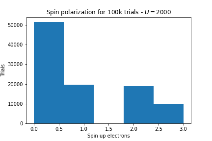
Now let’s check our earlier hypotheses:
- I set \(t = 1, U = 2000, \mu = 1\).
Here’s the number of spin-up electrons over 100,000 ground states:
- Now I set \(t=1000, U=2, \mu=1\).
Here’re the results:
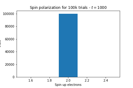
As we expected, as \(U \rightarrow \infty\) we get lots of local moments but as \(t \rightarrow \infty\) we get no local moments.